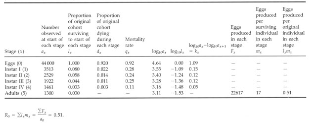
Table 1. A cohort life-table for the common grasshopper, Chorthippus brunneus (After Richards and Waloff 1954).
1. Describing population dynamics
There are a number of methods to describe populations from field measurements: dynamic and static life tables, and transition matrices. All are based on censusing individuals in groups, categorized according to their state (age, size, or stage). They are used to explain population dynamics in relation to demographic processes, and to predict the fate of the population.The methods differ in a) convenience of data collection, b) basic assumptions and c) the way they derive population growth rate. Because this also depends on the general biology and life cycle of the organism, some methods are better for some kinds of populations, but not for others.
Dynamic life tables describe survivorship and fecundity (production of eggs, seeds, or young) at different ages of a cohort (a sample of individuals recruited approximately at the same time). Usually the cohort is followed until the last member dies. Survivorship is calculated as the relative change in the number of individuals of the cohort between two successive censuses. The census is very simple, since individuals need only be recognized to differentiate them from other cohorts in the same population, and thus are only counted. No marking is needed, because for an individual to be counted means it survived since last census, and determines its age unambiguously. Transition models, as will be discussed later, require more elaborate censuses.
Age may be convenient to use in cohort studies, but it does not always play a primary role in the development and life cycle of the organisms. This is probably true for all plant and most animal taxa, except birds and mammals. The latter's determinate growth (an individually fixed adult size) and hormonal clock, combined with their ability to learn, make age a suitable attribute to describe population dynamics. In most other cases, size is biologically more important, as it determines resource acquisition, competitive ability, survivorship and sexual maturity and reproductive output. Only if size and age are strongly correlated in such a population, age may be preferable.
Stage is very useful in cohort studies of annual organisms if surviving organisms all pass through relatively short stages, so that stages hardly overlap (occur at the same time), and stage and age are correlated. This is the case in Richards and Waloff's (1954) study of grasshoppers (Table 1), cited in Begon et al. (1990). However, if size or stage is attained at different rates for different individuals in the population, as is often the case, they are not useful for constructing life tables. Then, transition models are more appropriate.
Table 1. A cohort life-table for the common grasshopper, Chorthippus
brunneus
(After Richards and Waloff 1954).
2. Survivorship
Two kinds of information are derived from these cohort studies:
survivorship
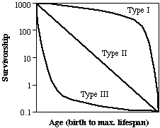
curves and population growth rates. Survivorship curves
show
how mortality varies with age of the individuals of the cohort. Age-specific
mortality, as well as age-specific fecundity, is due to
changing
susceptibilities and capabilities of the individual, and the variation
in its environmental exposure. Depending on the age at which most of
the
mortality takes place, organisms can have different survivorship
curves.
Deevey (1947) described three types of curves (Fig. 1):
Type I occurs
when survival of young is high, and mortality increases drastically
towards
the end of the lifespan. This is typical of very protected life styles.
In case of Type II survivorship curves, mortality is constant
with
age, as in a decay process. Most organisms have a Type III
curve,
where most individuals die when they are young, while older individuals
are good survivors.
3. Population growth rateFig. 1. Three types of survivorship curves (Begon et al. 1990, Deevey 1947).
Population growth rate of a cohort is defined as the basic reproductive rate R0 for a generation over its lifetime. Using dynamic life tables is best suited for semelparous animals or monocarpic plants, especially annual organisms, as in the study on the annual plant species Phlox drummondii by Leverich and Levin (1979) (Table 2). These have a single cohort per year, and thus have no overlapping generations. Perennial iteroparous/polycarpic organisms do have overlapping generations, which makes the method less straightforward, though often still useful. Connell (1970) used this method on the long-lived barnacle Balanus glandula (Table 3). Basic reproductive rate R0 measures the mean number of offspring that an individual of the cohort produces in its lifetime. Offspring denotes the number of individuals in the first stage of the life cycle (zygotes or young, depending on the organism).
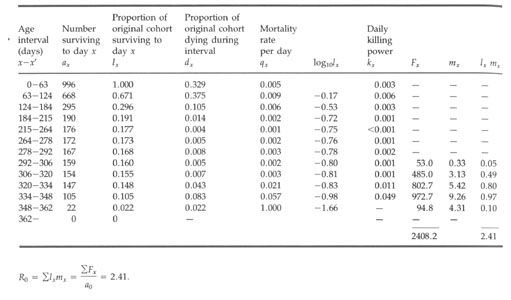
Table 2. A cohort life-table for Phlox drumondii (after
Leverich
and Levin 1979).
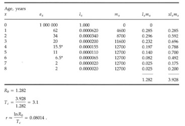
Table 3. A cohort life-table and fecundity schedule for the barnacle
Balanus
glandula at Pile Point, San Juan Island, Washington (Conell 1970).
(* - estimated by interpolation from the survivorship curve).
There are two ways to arrive at the basic reproductive rate. The first method is R0= ∑ F x /a0, where ∑ F x, the sum of the Fx's, is the number of offspring over the life span of the cohort, and a0 is the first stage. The ratio shows the relative change in population size/density from one generation of the cohort to the next. R0 is also measured as R0=∑ l x m x, the sum of l x, the chance of an individual surviving to age x (the time from the birth of the cohort to the census x, not necessarily in years), times m x, the number of offspring produced during the time from age x-1 to x. The advantage of this model is, that it is explicit about the relation between overall population growth and the actual demographic processes that take place through time in the cohort. For annual organisms this sequence of processes tracks the changing of the seasons.
In cohort studies, R0 is determined over the generation time. If the organism is an annual plant or animal, R0 also denotes population growth rate R, defined per year: R = R0. In perennial semelparous or monocarpic organisms, R0 should be corrected for generation time T (>1 year). Since R0=RT, so that lnR=(ln R0)/T. However, for organisms with overlapping generations, it is difficult to estimate annual growth rate accurately since generation time T is in fact unknown. Instead of T, R is given by (lnR=(ln R0)/Tc). R0 is corrected by Tc, the average cohort lifespan, which is the average time from the birth of an individual to the birth of one of its offspring, calculated as the sum of lengths of time of the offspring of all individuals divided by the total number of offspring:
Tc=( ∑x. lx m x)/ (∑ lx m x ) = (∑x. lx m x)/ R0.
The presence of three generations at the same time, i.e. if some individuals have produced offspring themselves while their parents are still alive, can not be incorporated in the equation.
4. Static life tables
A static life table contains the age groups in a population at one particular period of time. Thus, cohorts are not followed in time, but reconstructed using one-time observations. These can be used to calculate population growth only if an assumption is made. The assumption is that the mortality experienced by the cohort at any age stays constant in time. In other words, birth rates and age-specific survivorship are assumed to be independent of the actual year in which the observations are made. Only rarely is this assumption truly justified. Therefore, the conclusions tell us how a cohort should behave, if we would have observed it and if conditions are constant between years. An example is the study of red deer by Lowe (1969) (Table 4), described in Begon et al. (1990).
A second, less problematic application of static life tables is
using
them in order to reconstruct past events, as Crisp and Lange
(1976)
did with the desert shrub Acacia burkitii (Begon et al.
1990, page
144 and 145). They were able to show, among others, the effects of
grazing,
because they compared two stands using one as a control.
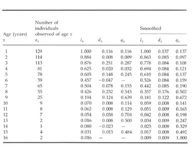
Table 4. A static life-table for red deer hinds on the island of Rhum,
based on the reconstructed age-structure of the population in 1957
(After
Lowe 1969).
References (* = required reading)
Connell, J. H., 1970. A predator-prey system in the marine intertidal region. I. Balanus glandula and several predatory species of Thais. Ecological Monographs 40: 49-78.
Crisp, M. D. and R. T. Lange, 1976. Age structure distribution and survival under grazing of the arid zone shrub Acacia burkitii. Oikos 27: 86-92.
Deevey, E. S., 1947. Life tables for natural populations of animals. Quarterly Review of Biology 22: 283-314.
* Leverich, W. J. and D. A. Levin, 1979. Age-specific survivorship and reproduction in Phlox drummondii. American Naturalist 113: 881-903.
Lowe, V. P. W., 1969. Population dynamics of the red deer (Cervus elaphus L.) on Rhum. Journal of Animal Ecology 38: 425-457.
Richards, O. W. and N. Waloff, 1954. Studies on the biology and population dynamics of British grasshoppers. Anti-Locust Bulletin 17: 1-182.